
Data matching algorithms determine whether two records refer to the same real-world entity. The right algorithm for a given field depends on the data type, error pattern, and acceptable false-positive rate — and most production record linkage systems combine three or more algorithms in a weighted scoring pipeline rather than relying on one.
This article walks through the core algorithms, how they compose into a multi-algorithm pipeline, and how to configure thresholds and weights for enterprise-grade accuracy.
Ready to see multi-algorithm matching in action? Start a free trial of Match Data Pro — no contract required.
Why a Single Algorithm Is Never Enough
Consider a typical customer record with five matchable fields: first name, last name, email, phone, and street address. Each field has a distinct error profile:
- Names suffer from nicknames (Bob vs. Robert), transpositions (Smth vs. Smith), and culturally variable ordering.
- Email addresses are largely exact — a single character difference almost always means a different mailbox.
- Phone numbers contain formatting noise (brackets, dashes, country codes) but consistent digit sequences.
- Addresses have abbreviation variants (St. vs. Street, Apt vs. Unit), missing suite numbers, and postal code errors.
A single Levenshtein edit-distance score applied uniformly across all five fields would over-penalise “St.” vs. “Street” (3 edits) while ignoring that “bob@acme.com” and “robert@acme.com” are plausibly the same person. The solution is to assign each field an algorithm matched to its error profile, then combine scores with field weights.
Before choosing algorithms, use AI-powered data profiling to measure the actual error distributions in your dataset — completeness rates, value cardinality, and common format variants — so your algorithm choices are evidence-based, not assumed.
The Core Data Matching Algorithms
1. Exact Match
Exact match compares two field values character-for-character. It is the fastest and most precise algorithm but has zero tolerance for variation. Use it for high-cardinality identifiers: tax IDs, email addresses after lowercasing, IBAN numbers, and national identity numbers. It should never be the only matching criterion on a record — even a single keystroke error will cause a miss.
2. Levenshtein Edit Distance
Levenshtein distance counts the minimum insertions, deletions, and substitutions needed to transform one string into another. “Smith” to “Smyth” costs 1 substitution; “Jon” to “John” costs 1 insertion. For short strings (names up to ~20 characters), this algorithm is highly effective. Raw distance is usually normalised to a similarity score: 1 − (distance / max_length), yielding a 0–1 range where 1.0 is identical. A threshold of 0.85 works well for surname matching in English-language datasets.
Levenshtein becomes expensive at scale because every pair requires an O(m×n) computation. Efficient fuzzy matching pipelines address this by applying blocking first — grouping records by a shared key (e.g. first three letters of surname plus ZIP code) before computing edit distances only within candidate pairs.
3. Jaro-Winkler
Jaro-Winkler is specifically designed for short strings and gives extra weight to prefix agreement, making it well-suited for given names and surnames. “MARTHA” and “MARHTA” (transposed characters) score 0.944 under Jaro-Winkler — much higher than pure Levenshtein would suggest — because the algorithm accounts for the cognitive reality of typing transpositions. Set a threshold of 0.88–0.92 for first-name matching; lower thresholds produce too many false positives with short names.
4. Soundex and Phonetic Algorithms
Soundex encodes a name as a letter plus three digits representing consonant sounds: “Robert” and “Rupert” both encode as R163. Double Metaphone and NYSIIS are more accurate phonetic algorithms that handle international names better. Phonetic matching is most useful as a blocking key — grouping records by sound before a more precise algorithm (Jaro-Winkler or Levenshtein) runs within each group. Do not use phonetics alone: “Smith” and “Schmidt” share phonetic similarity but are different surnames in most jurisdictions.
5. Token-Based Algorithms (Jaccard, TF-IDF)
Token-based algorithms split strings into tokens (words or n-grams) and measure set overlap. Jaccard similarity for “123 Main Street Apt 4B” vs. “123 Main St #4B” computes as shared tokens / union of tokens. This handles word-order variation and abbreviations better than edit-distance algorithms. TF-IDF weighting penalises common tokens (“Street”, “Avenue”) and rewards rare ones, making it useful for company name matching where generic words like “Inc.”, “LLC”, and “Corp.” appear in nearly every record.
See how fuzzy matching algorithms compare in practice across these dimensions, including configurable thresholds and field weights.
6. Numeric and Date Comparison
Phone numbers, ZIP codes, and dates require their own logic. For phone numbers, strip all non-digit characters first, then compare the resulting digit string exactly or with a 1–2 digit tolerance for transpositions. For dates, normalise to ISO 8601 before comparison and consider a date-transposition check (day/month swap): “1987-03-12” and “1987-12-03” differ by 10 edits but may represent the same person with a common entry error.
Building a Multi-Algorithm Weighted Scoring Pipeline
A production record linkage system scores each field independently and combines the scores using field weights. Here is an example weighted scoring configuration for a customer deduplication job:
| Field | Algorithm | Weight | Match Threshold |
|---|---|---|---|
| Email (normalised) | Exact | 0.35 | 1.0 |
| Apellido | Jaro-Winkler | 0.20 | 0.88 |
| First name | Jaro-Winkler | 0.15 | 0.85 |
| Phone (digits only) | Exact / 1-digit tolerance | 0.15 | 0.95 |
| Street address | Token Jaccard | 0.10 | 0.75 |
| ZIP code | Exact | 0.05 | 1.0 |
The composite score is the weighted sum of individual field scores. Pairs scoring above 0.85 are auto-matched; pairs between 0.70–0.85 go to a review queue; pairs below 0.70 are rejected. These thresholds are starting points — tune them using a labelled gold set of known matches and non-matches from your own data.
Deterministic vs. Probabilistic Matching
The weighted scoring approach described above is probabilistic — it assigns a match likelihood based on evidence strength. Deterministic matching, by contrast, applies explicit rules: “if email matches exactly, these records are the same entity.” Most production systems use both in sequence: deterministic rules handle the high-confidence cases quickly, and probabilistic scoring handles ambiguous cases. Learn how to configure deterministic vs. probabilistic matching for your specific data quality goals.
Blocking: Making Scale Practical
Comparing every record against every other record is an O(n²) operation. At 1 million records, that is 500 billion comparisons — infeasible at any reasonable compute cost. Blocking (also called candidate selection or pre-filtering) reduces the comparison space by grouping records that share at least one indexing key before running the full algorithm suite.
Common Blocking Strategies
- Sorted neighbourhood: Sort records by a blocking key (e.g. Soundex of surname), then compare each record only to its W nearest neighbours in the sorted list. Good for name-heavy deduplication.
- Prefix blocking: Group records by the first N characters of a field (e.g. first 4 characters of email domain). Simple and fast; misses records where the prefix itself is corrupted.
- Multi-pass blocking: Run three or four independent blocking passes with different keys (surname prefix, phone last 7 digits, postal code), then union the candidate pairs. Increases recall at the cost of more comparisons.
- LSH (Locality-Sensitive Hashing): Projects high-dimensional feature vectors into hash buckets so that similar records land in the same bucket with high probability. Used in ML-based matching pipelines.
Match Data Pro’s deduplication engine applies multi-pass blocking automatically, selecting blocking keys based on field completeness and cardinality scores from the profiling stage. This means you do not have to hand-craft blocking rules — the platform derives them from your data characteristics.
Entity Resolution: Closing the Loop on Multi-Source Matching
Record linkage within a single dataset — deduplication — is simpler than linking records across multiple source systems. Cross-system entity resolution must handle the case where Record A from CRM, Record B from ERP, and Record C from a marketing platform all represent the same customer but share no common identifier and have partially different field values.
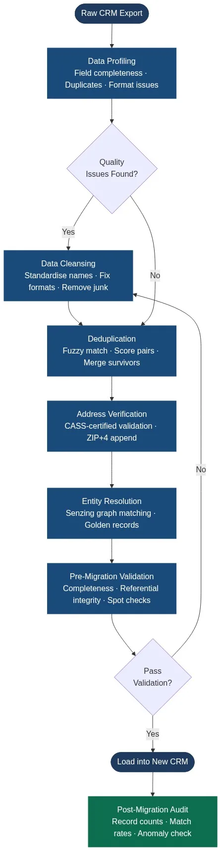
Graph-based entity resolution approaches this problem differently from pairwise scoring. Each record becomes a node; each candidate pair relationship with a score above a threshold becomes an edge. Connected components in the resulting graph identify entity clusters. Senzing entity resolution, integrated into Match Data Pro, uses this graph approach with pre-trained models that handle names, addresses, dates, and identifiers across jurisdictions without manual rule authoring.
Once entity clusters are resolved, survivorship rules determine which field values from the cluster members populate the golden record. Data match merging and survivorship rules cover this in detail — key decisions include source priority (trust CRM over web form submissions), recency (use the most recently updated value), and completeness (prefer non-null values from any source).
Configuring and Tuning Your Algorithm Stack
Every dataset needs tuning. A threshold of 0.88 on Jaro-Winkler that works well for an English-language customer database will produce false positives on a Spanish-language or Chinese-transliterated dataset. Here are the practical steps:
Paso 1: Perfile primero sus datos
Run AI data profiling to measure: field completeness, unique value rates, top-N value distributions, and pattern frequencies. A field with 40% null rate should carry a lower weight in composite scoring. A field where 90% of values share the same 3-character prefix is a bad blocking key.
Step 2: Cleanse Before You Match
Algorithm accuracy degrades on dirty input. Standardise before scoring: lowercase all text, strip punctuation from phone numbers, expand abbreviations (St. → Street, Blvd. → Boulevard), remove salutations from name fields. Data cleansing applied before matching reduces the algorithm workload and lowers false negative rates — a pair that would have scored 0.72 (below threshold) on raw data may score 0.91 after normalisation.
Step 3: Build a Gold Set
Label 500–2,000 record pairs as definite matches, definite non-matches, and uncertain. Use this set to measure precision and recall at different composite score thresholds. Plot a precision-recall curve and choose the operating point that matches your use case: a fraud detection pipeline tolerates low recall to keep precision at 99%; a customer 360 view tolerates some false positives to maximise recall.
Step 4: Iterate on Field Weights
Run the matching job against the gold set. Examine the false negatives (pairs that are true matches but scored below threshold): which fields are dragging the composite score down? Increase their weight or lower their individual threshold. Examine false positives similarly. Two or three iterations against the gold set typically converge on a stable configuration.
Match Data Pro supports configurable field weights, per-field algorithm selection, and multi-pass blocking through its job configuration UI — no code required. Book a demo to walk through threshold tuning on your own data sample.
Frequently Asked Questions
What is the best algorithm for matching names in a customer database?
Jaro-Winkler is the standard choice for name matching because it gives extra weight to prefix agreement and handles transpositions well. For surname matching with phonetic variation across cultural backgrounds, combine Jaro-Winkler with Double Metaphone as a blocking key. A threshold of 0.88–0.92 on Jaro-Winkler works well for most English-language customer datasets, but validate against a gold set from your own data.
How many algorithms should a record linkage pipeline use?
Most production pipelines use three to six algorithms, one per field type. More algorithms do not automatically improve accuracy; what matters is choosing the right algorithm for each field’s error profile and setting field weights based on discriminating power. Email and phone number exact matches carry much more weight than a partial name similarity score when assigning a composite match score.
What is blocking and why is it essential for large datasets?
Blocking reduces the candidate comparison space from O(n²) to manageable size by grouping records that share at least one indexing key. Without blocking, a 1 million record dataset requires 500 billion pairwise comparisons. With multi-pass blocking on three keys, the comparison space typically shrinks to under 5 million pairs — a 100,000x reduction — making full algorithm scoring computationally feasible.
When should I use deterministic matching vs. probabilistic matching?
Use deterministic matching when you have a reliable shared identifier (exact email, tax ID, IBAN) that makes the match decision unambiguous. Use probabilistic (weighted scoring) matching when no single field is trustworthy enough alone — which is the case for most real-world CRM deduplication scenarios. Most enterprise pipelines use deterministic rules first to handle the easy cases, then apply probabilistic scoring to the remainder.
How do I measure whether my matching configuration is accurate enough?
Build a labelled gold set of 500–2,000 record pairs — manually verified as matches or non-matches. Run your algorithm configuration against the gold set and compute precision (what fraction of flagged matches are correct) and recall (what fraction of true matches were found). An F1 score above 0.92 is a reasonable target for a production customer deduplication pipeline. Tune field weights and thresholds iteratively against the gold set until you reach your target.